Final Assessment >> Excel Skills for Business: Intermediate I

Final Assessment >> Excel Skills for Business: Intermediate I

1. Final assignment for Course 2In order to solve this assignment, please follow the steps below:
STEP 1: Download the Excel workbook, save it on your device and open it.

C2 Final Assessment.xlsx

STEP 2: Follow the instructions in order to answer the quiz questions. You will need to perform each task on your worksheet and then type in the solution into the Quiz answer boxes.
Good luck with this final assessment for the course. You have worked hard to get here. Trust your skills and get into it.
All the best,
Your Excel-Team
Here is your first question:
Have a look at the first 3 worksheets, they contain student marks for 3 terms. Now go to the Final Marks worksheet and use 3D-Formulas to get Benjamin Abbot’s class test average for terms 1, 2 and 4. Copy the formula across to I4 and then down for the rest of the students. What was the Average Final Mark (as shown in cell M4)?
Please enter the number with one decimal ##.#

62.6

2. Note that you have a sheet called Marks Term 3 but it is not in the right position. Move this sheet to sit between the sheets Marks Term 2 and Marks Term 4. Check the Final Marks Sheet, what is the average Final Mark now?
Please enter the number with one decimal ##.#

62.7

3. Select the range A3:J465 and use Create from Selection to name each of the columns of data. This should have corrected the missing stats figures. What was the median Final Mark (M5)?
Please enter the number with one decimal ##.#

63.8

4. Select the range L20:M26 and name it Grades. This should have corrected the grades calculations. What grade did Olivia Jones get?

C

5. In M10 use a formula to calculate the total number of Fail grades. Copy the formula down to M16. Note cell P4 which displays the Total Number of students who achieved a “C” should have changed colour. What colour is the cell?

• Yellow
• Blue
• Green
• Orange

6. In N10 create a mixed reference formula that will count how many of Mr Chang’s students got a Fail. Drag the formula down and across to complete the table. Observe P5, which shows the number of A’s achieved by Ms Sekibo’s students. It should have changed colour. What colour is it now?

• Green
• Blue
• Yellow
• Orange

7. Have a look at the worksheets Absences Term 1 through to Term 4, they contain a list of dates that students were absent. We need to create a summary showing a count of how many days each student was absent. Go to the Absence Report Sheet. Click in A4, and then use the Consolidate tool to consolidate the data on the other Absences sheets. The results look a bit odd, but that is because the count values have been formatted as dates. Change the formatting to General or Number. Sort the data by Total Absences. How many students were absent for more than 15 days?

3

8. Go to the Student Report worksheet. Some of the information still needs to be completed. Create a formula in D4 to return the Student’s full name, this should be First Name followed by a space and then Surname. The case must also be corrected so that all words start with a capital letter but everything else is in lower case e.g., Benjamin Abbot. Copy the formula down for all the other students. What is the value of the check digit in S4?

662

9.In E4 create a formula to generate the student email address. This should be their first initial, followed by their surname, followed by “@newcollege.com”, and must all be in lower case, e.g. [email protected]. Copy the formula down for all the other students. What is the value of the check digit in S5?

311

10. The last two digits of the student number indicate the year the student enrolled. In F4 create a formula that will put “20” followed by the last two digits of the Student ID, e.g. 2015. Copy the formula down for all the other students. What is the value of the check digit in S6?

242

11. We would like to get an idea of how students have progressed over the year. Click in M4 and create a sparkline line chart that charts the data in cells I4:L4. Copy the sparkline down for all the other students. Change the sparkline to show the highest point. Which of these sparklines represents Olivia Jones’ data?

• This:

• This:

• This:

• This:

12. Convert the data in the Student Report Sheet to a table. Name the table Report and change the style to Green Table Style Medium 21. Which of the following styles did you choose?

• This:

• This:

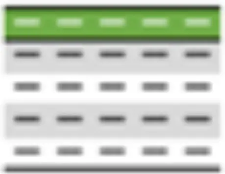
• This:

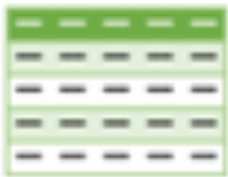
• This:

13. With the table still selected, turn on the Total Row. What are the Total Fees Owing?
Don’t enter the currency symbol, just the number and decimal places, e.g. #######.##

3451742.00

14. In the Total Row in the Year Enrolled column, chose the correct function to calculate the number of all students enrolled. How many are there?

462

15. Filter the table to show all Distance Learning students who owe more than $9,000. How many are there?

41

16. We would like to compare the results for different types of students. Clear all filters. Use the data in the table to create a pivot table (in a new sheet) that shows Grade in the Row Labels, Student Type in the Column Labels, and Count of Grade in the Values section. How many A’s did the Part Time Students get?

33

17. Change the pivot to show the values as a percentage of the column total. What percentage of Part Time students failed?
Don’t enter the percentage symbol, please just enter the number as ##.## (2 decimal places).

12.88

18. Mr Chang has observed that the students attending the college seem to be increasingly more able and more motivated. He would like to see if there is a pattern in the results based on enrolment date. Click in A17 and create another pivot table to show the average final mark by enrolment date. Add a filter field and change the filter to only show data for Mr Chang. Format the values to only show 2 decimal places. What was the Average mark for 2017?
Please enter the number with two decimal places.

68.05

19. Create a Clustered Column pivot chart using the data in the second pivot table (if you have Excel for Mac select the data in A17:B20 and just create a regular chart). Add a linear trendline and display the R-squared value on the chart. What is the R-squared value?
Please enter the number as #.#### (4 decimal places).

0.9481

20. Have a look at the other trend line options and select the one that returns the best R-squared value. Forecast forward for 1 period. If the trend continues, students who enrol in 2018 are expected to get an average result closest to…

• 68
• 70
• 73
• 76