Test your Skills: Summarising Data >> Excel Skills for Business: Intermediate I
1. The attached workbook is needed to answer all the questions associated with this quiz.
C2 W4 Assessment Workbook.xlsx
Use Create from Selection to name each of the columns of data in the Ealing Property Sales sheet.
Check the Name Box to see all your named ranges have been created correctly. What name has been applied to the data in Column D?
- YearSold
- Year Sold
- Year_Sold
- Year-Sold
2. In C3 use a COUNT function to count the values in the named range ID.
What answer does the COUNT function return?
Please enter just the number.
9
3. This is not the result we were hoping for, look carefully at the ID column, can you see why we got this answer?
Which function should you use if you wanted to pick up all the IDs?
- COUNTIF
- COUNTA
- COUNTIFS
- SUMIFS
4. Have a look at column J (Flat Number), note that a lot of the cells are blank.
Which function would you use to count the number of blank cells in a column?
Please enter just the function name all in UPPERCASE letters with no equal sign, brackets or arguments.
COUNTBLANK
5. On the Summary Data sheet, in cell B4, use a function to sum the Price Paid for all properties of type Terraced. Copy the formula down.
What was the total Price Paid for Flats?
Don’t enter the currency symbol or decimal points, just the plain number of the format #####
2393400
6. In C4 create a formula to sum the total Price Paid for all Terraced properties sold in 2014. Make any necessary adjustments and then drag the formula down and across to complete the table.
Which of these formulas is correct?
- =SUMIFS(Price_Paid,Property_Type,A4,Year_Sold,$C$3)
- =SUMIFS(Price_Paid,Property_Type,$A$4,Year_Sold,C3)
- =SUMIFS(Price_Paid,Property_Type,$A$4,Year_Sold,C$$3)
- =SUMIFS(Price_Paid,Property_Type,$A4,Year_Sold,C$3)
7. In F4 create a sparklines showing the sales trends for terraced houses from 2014 to 2016. Copy the sparkline down to F8.
Which of these property types follows a completely different trend to the others?
- Other
- Detached
- Semi
- Flat
8. Click in A12. Note the drop down that allows you to select different Towns, leave it set to London. In B13 create a calculation that will show the number of properties sold in the selected town for July 2015. (Note you will need to add criteria to check Year Sold and Month Sold). Copy the formula down to get results for the other months.
Which Month had the lowest number of sales?
Type out the full name of the month.
NOVEMBER
9. In C13 create a formula to sum the total price paid for properties sold in the selected region (London) for July 2015. (Note you will need to add criteria to check Year Sold and Month Sold.) Copy the formula down to get results for the other months.
Which Month had the second lowest total sales?
Type out the full name of the month.
10. Select the range A12:C18 and create a line chart. Put the Total Sales series on a secondary axis and change it to a Clustered Column chart.
Which of the following most closely resembles your chart?
- This one:

- This one:
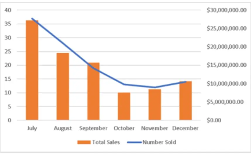
- This one:
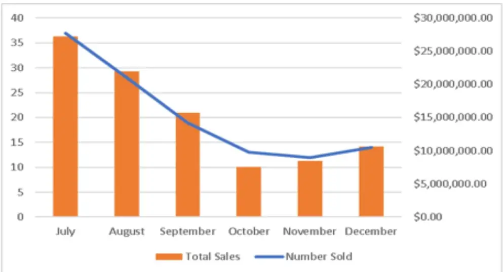
11. In your new chart select the Number Sold series and add a trend line. Show the R² value. Compare the results you get from the different trend line options.
Which of the following trendline options yields the best R² value?
- Exponential
- Linear
- Logarithmic
- Power
12. Change your trendline to a Polynomial Order 2.
What R² value does the Polynomial Order 2 show?
Type 0. followed by 4 digits e.g. 0.6789.
0.9933